FAQ Number 4

Does Risk-Neutral Valuation Mean that Investors Are Risk-Neutral?
What Is the Difference Between Real Simulation and Risk-Neutral Simulation?

Answers and example for geometric Brownian motion (GBM):

• Risk-neutral valuation (RNV) does not assume investors or firms with risk-neutral preferences;
• RNV does not use real probabilities. It uses risk neutral probabilities (“martingale measure”);
• Real simulation: real probabilities, it uses real drift a;
• Risk-neutral simulation: the sample paths are risk-adjusted.
  It uses a risk-neutral drift: a’ = r - d

The real simulation of a GBM uses the real drift a. The price at future time t is given by:

• By sampling the standard Normal distribution N(0, 1) you get the values for P_t;
• With real drift use the underlying asset (P) risk-adjusted discount rate r

The risk-neutral simulation of a GBM uses the risk-neutral drift a’ = r - d . The price at t is:

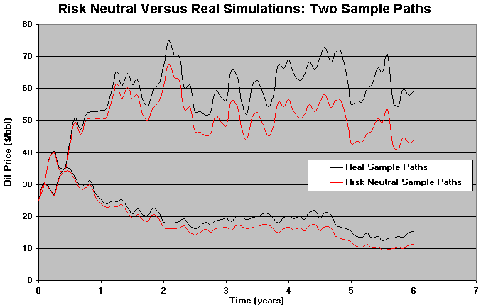
The chart below illustrates the difference of risk-neutral and real simulation by showing two sample paths for each type of simulation:

Note in the chart that the paths are parallel, and the risk neutral one is a risk premium lower than real sample path. This issue is because the risk neutral drift is equivalent to subtract a risk premium from the drift (see Trigeorgis' textbook, 1996, p.102):

Where l is the underlying asset market premium of risk in the sense that r = a + d = r + ls, (r = risk-adjusted discount rate for the underlying asset).

Example: European Real Options Value Using Simulation

Suppose a real options problem can approximately be represented by an European type call option (for additional discussion of this example, see the Monte Carlo page, section on European real options).

The first step is to simulate risk-neutral sample paths for the underlying asset (project value or commodity price) and take the cross-section distribution at the expiration T. You get the risk neutral distribution for the underlying asset.
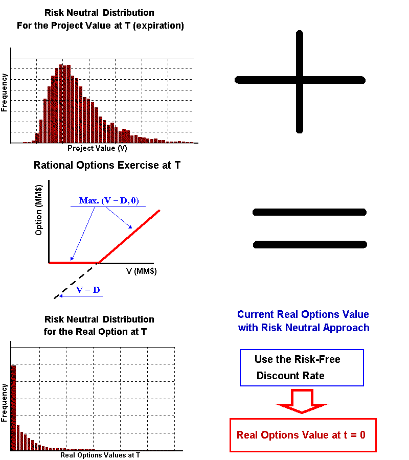
The figure below illustrates:

With the risk-neutral distribution of the project value V at the expiration (T), you can apply the options thinking: rational managers will exercise the option only if get positive expected values:
F (T)= max. (NPV, 0). This asymetric risk-neutral distribution for the European-type real options at T displaces the expected value to the higher value and represents the active management of real options.
The current value of the real options in this case is just to take the present value using the risk-free discount rate. The figure below shows this process.

Summary of Real versus Risk-Neutral Simulation/Valuation:

For the underlying asset, you get the same value:

• Simulating with real drift and discounting with risk-adjusted discount rate r ( where r = a + d );
• Or simulating with risk-neutral drift (r - d) but discounting with the risk-free interest rate (r)

For the option/derivative, the same is not true:

• Risk-neutral simulation gives the correct option result (discounting with r) but the real simulation does not gives the correct value (discounting with r);
• Why? Because the risk-adjusted discount rate is “adjusted” to the underlying asset, not to the option!

Risk-neutral valuation is based on the absence of arbitrage, portfolio replication (complete market).

• Incomplete markets: see next FAQ.